Python Tutorial 2: Making Maps
If you have followed the first EM-DAT Python Tutorial 1 or are already familiar with pandas and matplotlib, this second tutorial will show you basic examples on how to make maps with the EM-DAT data using the geopandas Python package.
Note: The Jupyter Notebook version of this tutorial is available on the EM-DAT Python Tutorials GitHub Repository.
Import Modules
Let us import the necessary modules and print their versions. For this tutorial, we used pandas v.2.1.1, geopandas v.0.14.3, and matplotlib v.3.8.3. If your package versions are different, you may have to adapt this tutorial by checking the corresponding package documentation.
import pandas as pd #data analysis package
import geopandas as gpd
import matplotlib as mpl
import matplotlib.pyplot as plt #plotting library
for i in [pd, gpd, mpl]:
    print(i.__name__, i.__version__)
pandas 2.2.1
geopandas 0.14.3
matplotlib 3.8.3
Creating a World Map
To create a world map, we need the EM-DAT data and a shapefile containing the country geometries.
EM-DAT: We download and load the EM-DAT data using pandas.
Country Shapefile: We download a country shapefile from Natural Earth Data. For a world map, we download the low resolution 1:110m Adimin 0 - Countries (last accessed: March 10, 2024) and unzip it.
Load and Filter EM-DAT
Let us load EM-DAT and filter it to make a global map of Earthquake disasters between 2000 and 2023. We calculate the number of unique identifiers (DisNo.) per country (ISO) We refer to the standard ISO column instead of the Country column of the EM-DAT Public Table to be able to make a join with the country shapefile.
df = pd.read_excel('public_emdat_2024-01-08.xlsx')
earthquake_counts = df[
    (df['Disaster Type'] == 'Earthquake') &
    (df['Start Year'] < 2024)
].groupby('ISO')["DisNo."].count().reset_index(name='EarthquakeCount')
earthquake_counts
| ISO | EarthquakeCount | |
|---|---|---|
| 0 | AFG | 21 |
| 1 | ALB | 4 |
| 2 | ARG | 2 |
| 3 | ASM | 1 |
| 4 | AZE | 3 |
| ... | ... | ... |
| 86 | USA | 10 |
| 87 | UZB | 1 |
| 88 | VUT | 2 |
| 89 | WSM | 1 |
| 90 | ZAF | 2 |
91 rows × 2 columns
Load the Country Shapefile
We use the gpd.read_file method to load the country shapefile and parse it into a geodataframe. A geodataframe is similar to a pandas dataframe, extept that has a geometry column.
We provide the filename argument, which is either a file name if located in the same directory than the running script, or a relative or absolute path, if not. In our case the shapefile with the .shp extension is located in the ne_110m_admin_0_countries folder.
Since the geodataframe contains 169 columns, we only keep the two column that we are interrested in, i.e., ISO_A3 and geometry.
gdf = gpd.read_file ('ne_110m_admin_0_countries/ne_110m_admin_0_countries.shp') # <-- Change path if necessary
gdf = gdf[['ISO_A3', 'geometry']]
gdf
Cannot find header.dxf (GDAL_DATA is not defined)
| ISO_A3 | geometry | |
|---|---|---|
| 0 | FJI | MULTIPOLYGON (((180.00000 -16.06713, 180.00000... |
| 1 | TZA | POLYGON ((33.90371 -0.95000, 34.07262 -1.05982... |
| 2 | ESH | POLYGON ((-8.66559 27.65643, -8.66512 27.58948... |
| 3 | CAN | MULTIPOLYGON (((-122.84000 49.00000, -122.9742... |
| 4 | USA | MULTIPOLYGON (((-122.84000 49.00000, -120.0000... |
| ... | ... | ... |
| 172 | SRB | POLYGON ((18.82982 45.90887, 18.82984 45.90888... |
| 173 | MNE | POLYGON ((20.07070 42.58863, 19.80161 42.50009... |
| 174 | -99 | POLYGON ((20.59025 41.85541, 20.52295 42.21787... |
| 175 | TTO | POLYGON ((-61.68000 10.76000, -61.10500 10.890... |
| 176 | SSD | POLYGON ((30.83385 3.50917, 29.95350 4.17370, ... |
177 rows × 2 columns
Important Notice: Above, some geometries do not have a ISO code, such as the one at row 174. Below, you will see that some ISO in EM-DAT are not matched with a geometries. Beyond this basic tutorial, we advice to carefully evaluate these correspondance and non-correspondance between ISO codes and to read the EM-DAT Documentation about ISO codes.
Join the Two Datasets
Let us merge the two dataset with an outer join, using the merge method. We prefer an outer join to keep the geometries of countries for which EM-DAT has no records.
earthquake_counts_with_geom = gdf.merge(
    earthquake_counts, left_on='ISO_A3', right_on='ISO', how='outer')
earthquake_counts_with_geom
| ISO_A3 | geometry | ISO | EarthquakeCount | |
|---|---|---|---|---|
| 0 | -99 | MULTIPOLYGON (((15.14282 79.67431, 15.52255 80... | NaN | NaN |
| 1 | -99 | MULTIPOLYGON (((-51.65780 4.15623, -52.24934 3... | NaN | NaN |
| 2 | -99 | POLYGON ((32.73178 35.14003, 32.80247 35.14550... | NaN | NaN |
| 3 | -99 | POLYGON ((48.94820 11.41062, 48.94820 11.41062... | NaN | NaN |
| 4 | -99 | POLYGON ((20.59025 41.85541, 20.52295 42.21787... | NaN | NaN |
| ... | ... | ... | ... | ... |
| 185 | NaN | None | WSM | 1.0 |
| 186 | YEM | POLYGON ((52.00001 19.00000, 52.78218 17.34974... | NaN | NaN |
| 187 | ZAF | POLYGON ((16.34498 -28.57671, 16.82402 -28.082... | ZAF | 2.0 |
| 188 | ZMB | POLYGON ((30.74001 -8.34001, 31.15775 -8.59458... | NaN | NaN |
| 189 | ZWE | POLYGON ((31.19141 -22.25151, 30.65987 -22.151... | NaN | NaN |
190 rows × 4 columns
Make the Map
To make the map, we use the geopandas built-in API, through the plot method built on the top of matplotlib.
Below, we show an hybrid plotting approach and first create an empty figure fig and ax object with matplotlib before passing the ax object as an argument within the plot method. This approach gives more control to users familiar with matplotlib to further customize the chart.
fig, ax = plt.subplots(figsize=(8,3))
earthquake_counts_with_geom.plot(
    column='EarthquakeCount',
    ax=ax,
    cmap='Reds',
    vmin=1,
    legend=True,
    legend_kwds={"label": "Nb of EM-DAT Earthquake"},
    missing_kwds= dict(color = "lightgrey",)
)
_ = ax.set_xlabel('Lon.')
_ = ax.set_ylabel('Lat.')
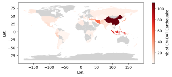
Output plot
Creating a Map at Admin Level 1
We can create a more detailed map using the Admin Units column in the EM-DAT Public Table. This column contains the identifiers of administrative units of level 1or 2 as defined by the Global Administrative Unit Layer (GAUL) for country impacted by non-biological natural hazards.
Similarly to the country map, we need to download a file containing GAUL geometries. The file corresponds to the last version of GAUL published in 2015. In this tutorial, we will focus on Japanese earthquake occurrence in EM-DAT.
Note: the file size is above 1.3Go and requires a performant computer to process in Python. Using a Geographical Information Software (GIS) for the preprocessing is another option.
Load the Admin Units Geopackage
The file is a geopackage .gpkg that contains multiple layers. Let us first describe these layers with the fiona package, which is a geopandas dependency.
import fiona
print(fiona.__name__, fiona.__version__)
for layername in fiona.listlayers('gaul2014_2015.gpkg'):
    with fiona.open('gaul2014_2015.gpkg', layer=layername) as src:
        print(layername, len(src))
fiona 1.9.5
level2 38258
level1 3422
level0 277
- The
level0layer contains the country geometries defined in GAUL. - Here, we make a map at the
level1. - Still, we need to load the administrative
level2because theAdmin Unitscolumn may refer to Admin 2 levels without mentionning the corresponding Admin 1 level. - Given the high size the admin 2 layer, we filter the data about Japan and overwrite our geodataframe variable to save memory.
gaul_adm2 = gpd.read_file ('gaul2014_2015.gpkg', layer='level2')
gaul_adm2 = gaul_adm2[gaul_adm2['ADM0_NAME'] == 'Japan']
gaul_adm2.info()
<class 'geopandas.geodataframe.GeoDataFrame'>
Index: 3348 entries, 23205 to 26552
Data columns (total 13 columns):
 #   Column      Non-Null Count  Dtype
---  ------      --------------  -----
 0   ADM2_CODE   3348 non-null   int64
 1   ADM2_NAME   3348 non-null   object
 2   STR2_YEAR   3348 non-null   int64
 3   EXP2_YEAR   3348 non-null   int64
 4   ADM1_CODE   3348 non-null   int64
 5   ADM1_NAME   3348 non-null   object
 6   STATUS      3348 non-null   object
 7   DISP_AREA   3348 non-null   object
 8   ADM0_CODE   3348 non-null   int64
 9   ADM0_NAME   3348 non-null   object
 10  Shape_Leng  3348 non-null   float64
 11  Shape_Area  3348 non-null   float64
 12  geometry    3348 non-null   geometry
dtypes: float64(2), geometry(1), int64(5), object(5)
memory usage: 366.2+ KB
The Admin 2 geodataframe has 12 columns describing the 3348 level 2 administrative units in Japan.
Filter EM-DAT Data
df_jpn = df[
    (df['ISO'] == 'JPN') &
    (df['Disaster Type'] == 'Earthquake') &
    (df['Start Year'] < 2024)
][['DisNo.', 'Admin Units']]
df_jpn
| DisNo. | Admin Units | |
|---|---|---|
| 392 | 2000-0428-JPN | [{"adm2_code":36308,"adm2_name":"Koodusimamura... |
| 610 | 2000-0656-JPN | [{"adm1_code":1680,"adm1_name":"Okayama"},{"ad... |
| 1013 | 2001-0123-JPN | [{"adm1_code":1654,"adm1_name":"Ehime"},{"adm1... |
| 2791 | 2003-0249-JPN | [{"adm1_code":1652,"adm1_name":"Akita"},{"adm1... |
| 2884 | 2003-0354-JPN | [{"adm2_code":35135,"adm2_name":"Hurukawasi"},... |
| 3014 | 2003-0476-JPN | [{"adm1_code":1661,"adm1_name":"Hokkaidoo"}] |
| 3824 | 2004-0532-JPN | [{"adm1_code":1690,"adm1_name":"Tookyoo"},{"ad... |
| 4182 | 2005-0129-JPN | [{"adm1_code":1656,"adm1_name":"Hukuoka"}] |
| 4253 | 2005-0211-JPN | [{"adm1_code":1656,"adm1_name":"Hukuoka"},{"ad... |
| 5769 | 2007-0101-JPN | [{"adm1_code":1678,"adm1_name":"Niigata"},{"ad... |
| 5912 | 2007-0258-JPN | [{"adm1_code":1675,"adm1_name":"Nagano"},{"adm... |
| 6311 | 2007-0654-JPN | [{"adm1_code":1672,"adm1_name":"Mie"},{"adm1_c... |
| 6606 | 2008-0242-JPN | [{"adm1_code":1652,"adm1_name":"Akita"},{"adm2... |
| 6637 | 2008-0275-JPN | [{"adm2_code":33543,"adm2_name":"Hatinohesi"}] |
| 7335 | 2009-0320-JPN | [{"adm1_code":1690,"adm1_name":"Tookyoo"},{"ad... |
| 8403 | 2011-0082-JPN | [{"adm1_code":1652,"adm1_name":"Akita"},{"adm1... |
| 8447 | 2011-0130-JPN | [{"adm1_code":1695,"adm1_name":"Yamagata"},{"a... |
| 9596 | 2013-0127-JPN | [{"adm1_code":1662,"adm1_name":"Hyoogo"}] |
| 10468 | 2014-0465-JPN | [{"adm2_code":35261,"adm2_name":"Hakubamura"}] |
| 11276 | 2016-0107-JPN | [{"adm1_code":1670,"adm1_name":"Kumamoto"}] |
| 11291 | 2016-0121-JPN | [{"adm1_code":1670,"adm1_name":"Kumamoto"},{"a... |
| 11631 | 2016-0492-JPN | [{"adm2_code":36364,"adm2_name":"Kurayosisi"}] |
| 12449 | 2018-0183-JPN | [{"adm1_code":1662,"adm1_name":"Hyoogo"},{"adm... |
| 12589 | 2018-0330-JPN | [{"adm2_code":34179,"adm2_name":"Atumatyoo"},{... |
| 13030 | 2019-0322-JPN | [{"adm1_code":1664,"adm1_name":"Isikawa"},{"ad... |
| 13949 | 2021-0105-JPN | [{"adm2_code":33868,"adm2_name":"Namiemati"}] |
| 14005 | 2021-0194-JPN | [{"adm1_code":1651,"adm1_name":"Aiti"},{"adm1_... |
| 14584 | 2022-0153-JPN | NaN |
| 15236 | 2023-0279-JPN | NaN |
Note: The last two events were not geolocated at a higher administrative levels.
Convert Admin 2 units to Admin 1 units
We create a python function, json_to_amdmin1, to extract the administrative level 1 codes from the Admin Units column of EM-DAT, based on the ADM1_CODE and ADM2_CODE of the Japan geodataframe.
import json

def json_to_admin1(json_str, gdf):
    """
    Convert a JSON string to a set of administrative level 1 codes.

    Parameters
    ----------
    json_str
        A JSON string representing administrative areas, or None.
    gdf
        A GeoDataFrame containing administrative codes and their corresponding
        levels.

    Returns
    -------
    A set of administrative level 1 (ADM1) codes extracted from the input JSON.

    Raises
    ------
    ValueError
        If the administrative code is missing from the input data or ADM2_CODE
        not found in the provided GeoDataFrame.

    """
    adm_list = json.loads(json_str) if isinstance(json_str, str) else None
    adm1_list = []
    if adm_list is not None:
        for entry in adm_list:
            if 'adm1_code' in entry.keys():
                adm1_code = entry['adm1_code']
            elif 'adm2_code' in entry.keys():
                gdf_sel = gdf[gdf['ADM2_CODE'] == entry['adm2_code']]
                if not gdf_sel.empty:
                    adm1_code = gdf_sel.iloc[0]['ADM1_CODE']
                else:
                    raise ValueError(
                        'ADM2_CODE not found in the provided GeoDataFrame.'
                    )
            else:
                raise ValueError(
                    'Administrative code is missing from the provided data.'
                )
            adm1_list.append(adm1_code)
    return set(adm1_list)
We apply the function to all elements of the Admin Units column.
df_jpn.loc[:, 'Admin_1'] = df_jpn['Admin Units'].apply(
    lambda x: json_to_admin1(x, gaul_adm2))

df_jpn[['Admin Units', 'Admin_1']]
| Admin Units | Admin_1 | |
|---|---|---|
| 392 | [{"adm2_code":36308,"adm2_name":"Koodusimamura... | {1690} |
| 610 | [{"adm1_code":1680,"adm1_name":"Okayama"},{"ad... | {1680, 1691, 1686} |
| 1013 | [{"adm1_code":1654,"adm1_name":"Ehime"},{"adm1... | {1660, 1654} |
| 2791 | [{"adm1_code":1652,"adm1_name":"Akita"},{"adm1... | {1665, 1673, 1652, 1653, 1695} |
| 2884 | [{"adm2_code":35135,"adm2_name":"Hurukawasi"},... | {1673} |
| 3014 | [{"adm1_code":1661,"adm1_name":"Hokkaidoo"}] | {1661} |
| 3824 | [{"adm1_code":1690,"adm1_name":"Tookyoo"},{"ad... | {1690, 1678} |
| 4182 | [{"adm1_code":1656,"adm1_name":"Hukuoka"}] | {1656} |
| 4253 | [{"adm1_code":1656,"adm1_name":"Hukuoka"},{"ad... | {1656, 1683} |
| 5769 | [{"adm1_code":1678,"adm1_name":"Niigata"},{"ad... | {1664, 1692, 1678} |
| 5912 | [{"adm1_code":1675,"adm1_name":"Nagano"},{"adm... | {1675, 1692, 1678} |
| 6311 | [{"adm1_code":1672,"adm1_name":"Mie"},{"adm1_c... | {1672, 1677, 1685} |
| 6606 | [{"adm1_code":1652,"adm1_name":"Akita"},{"adm2... | {1665, 1673, 1652} |
| 6637 | [{"adm2_code":33543,"adm2_name":"Hatinohesi"}] | {1653} |
| 7335 | [{"adm1_code":1690,"adm1_name":"Tookyoo"},{"ad... | {1690, 1687} |
| 8403 | [{"adm1_code":1652,"adm1_name":"Akita"},{"adm1... | {1665, 1668, 1693, 1673, 1675, 1695, 1652, 165... |
| 8447 | [{"adm1_code":1695,"adm1_name":"Yamagata"},{"a... | {1673, 1695} |
| 9596 | [{"adm1_code":1662,"adm1_name":"Hyoogo"}] | {1662} |
| 10468 | [{"adm2_code":35261,"adm2_name":"Hakubamura"}] | {1675} |
| 11276 | [{"adm1_code":1670,"adm1_name":"Kumamoto"}] | {1670} |
| 11291 | [{"adm1_code":1670,"adm1_name":"Kumamoto"},{"a... | {1674, 1683, 1670} |
| 11631 | [{"adm2_code":36364,"adm2_name":"Kurayosisi"}] | {1691} |
| 12449 | [{"adm1_code":1662,"adm1_name":"Hyoogo"},{"adm... | {1682, 1677, 1662, 1671} |
| 12589 | [{"adm2_code":34179,"adm2_name":"Atumatyoo"},{... | {1661} |
| 13030 | [{"adm1_code":1664,"adm1_name":"Isikawa"},{"ad... | {1664, 1673, 1678, 1695} |
| 13949 | [{"adm2_code":33868,"adm2_name":"Namiemati"}] | {1657} |
| 14005 | [{"adm1_code":1651,"adm1_name":"Aiti"},{"adm1_... | {1664, 1665, 1668, 1671, 1672, 1673, 1675, 167... |
| 14584 | NaN | {} |
| 15236 | NaN | {} |
Count Earthquakes per Admin 1 Units
The can be done applying the explode method on the new Admin_1 column. The method will add rows based on the number of Admin 1 we have in each set inside the Admin_1 column. Then the counting can be performed using the former groupby approach.
count_per_adm1 = df_jpn.explode('Admin_1').groupby(
    'Admin_1')['DisNo.'].count().rename('EQ Count')
count_per_adm1.head()
Admin_1
1651    1
1652    4
1653    4
1654    1
1655    1
Name: EQ Count, dtype: int64
Recreate the Admin 1 Layer
Since the Japan geodataframe contains the admin2 geometries, we could load the Admin 1 layer or simply dissolve the geometries based on the ADM1_CODE column. The geopandas package is equipped with the dissolve method.
gdf_jpn_adm1 = gaul_adm2.dissolve(by='ADM1_CODE')
gdf_jpn_adm1.plot()
<Axes: >
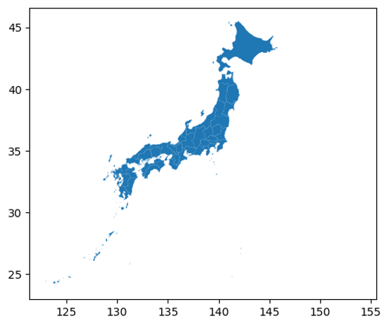
Output plot
Join the Two Datasets
Again, we can use the merge method to join the datasets together, here, based on their index.
gdf_jpn_adm1_merged = gdf_jpn_adm1.merge(count_per_adm1,
                                         left_index=True,
                                         right_index=True,
                                         how='outer')
Make the Map
fig, ax = plt.subplots()

gdf_jpn_adm1_merged.plot(
    column='EQ Count', cmap='YlOrRd',
    linewidth=0.8, ax=ax,edgecolor='0.8',
    legend=True,
    legend_kwds={'label': "Earthquake Count in EM-DAT"}
)
_ = ax.set_xlabel('Longitude')
_ = ax.set_ylabel('Latitude')
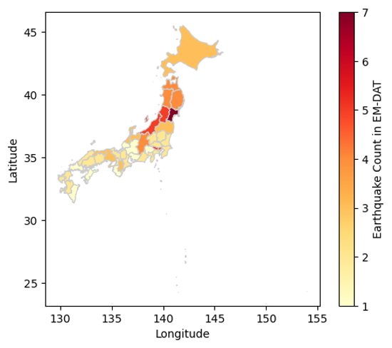
Output plot
We have just covered the basics on how to join the EM-DAT pandas DataFrame with a geopandas GeoDataFrame to make maps. To delve further into your analyses, we encourage you to continue your learning of geopandas, matplotlib, or, in particular, cartopy for more advanced map customization, with the many resources available online.